Scrap Your Moving Average Forecast! Improve Forecasting Performance with a NaïveLT Benchmark for Leadtime Demand Forecasting 15 Nov 2020, 7:05 pm

Assessing forecasting performance for lead-time demand forecasts has been a topic herebefore. A lead-time forecast is commonly used in practice for intermittent and regular demand forecasting applications, when 

• planning product mix based on future patterns of demand at the item, product group and store level
• setting safety stock levels for SKUs at multiple locations
• evaluating accuracy in S&OP and annual budget planning meetings
• validating performance standardsin forecasting competitions

In contrast to multi one-step ahead or short-term forecasts, a lead-time forecast is a multi-step ahead forecast with a fixed horizon. It has always been a difficult and challenging task for demand planners and managers.

In several previous articles, I used a dataset (shown below) to assess forecasting performance with the test or holdout data (in italics) in the row for year 2016. 

For a twelve-month holdout sample (Sep 2016 – Aug 2017), I have created three forecasts by using (1) judgment, (2) a method and (3) a statistical model. For a judgment forecast, I used previous year actuals (Sep 2015 – Aug 2016) as the forecast for the hold-out sample year. This forecast profile is labeled Year-1. Thisis also known as the Naive12 method. For a method forecast, I use the level point- forecast (MAVG_12), which is simply the average of previous 12-months of history repeated over the forecast horizon. The model forecast is based on the State Space forecasting model ETS (A,A,M), which is an exponential smoothing model with a local level and multiplicative seasonal forecast profile as described in Chapter 8 of my book Change&Chance Embraced.

View Lead-time Forecasts as Forecast Profiles Rather Than a Sequence of Point Forecasts

For lead-time forecasts, we can assess the performance of forecast profiles and create objective measures of accuracy and skill performance with information theoretic concepts for performance measurement.

The actuals and lead-time forecasts in the respective lead-time forecasts are coded or transformed into alphabet profiles AAP (Actual Alphabet Profile) and FAPs (Forecast Alphabet Profile) by dividing a lead-time Total into each component of the respective profiles. Coding results in positive fractions (weights) that sum to one, and have the same property as a discrete probability distribution. You can see that this does not change the pattern of the original profile.

Data Quality Matters Because Bad Data Will Beat a Good Forecast Every Time

It is not only a best practice, but should be a necessary requirement for demand planners to first explore and improve the quality of data prior to forecast modeling. .In the italicized row for year 2016, there appear to be unusual values in period 4 (Dec) and period 5 (January). You can also see it in the graph as the AAP peaks one period after the FAPs.

By switching Dec 2016 (= 49786) with Jan 2017 (= 73069), the seasonal pattern in the holdout sample is more consistent with its history. A preliminary analysis of variance for the seasonal and trend variation in these four years suggests that making the adjustment is important. The seasonal contribution to the total variation increased from 48% to 68%, appearing more consistent with the seasonality in the historical data and what might be expected in future years.

Introducing the NaïveLT Benchmark Forecast

A Naïve LT Benchmark can serve as a better benchmark than either the Year-1 naïve judgment forecast or MAVG-12 constant level method. The Naïve LT benchmark is the forecast to beat, so that we can use it to measure the effectiveness of the forecasting process demonstrating how much the method, model or judgmental forecast contributes to the benefit of the overall forecasting process.

The forecast alphabet profile (FAP) for the Naïve LT benchmark is a very straightforward calculation, simply the average of the individual FAPs in the history; in this case Year-1naive, Year-2 naive and Year-3 naive. They have the same pattern as the lead time forecast profiles in a Tier chart below. Note that creating the FAPs does not alter the pattern in the Tier chart, it only rescales them. In order to determine how effective the Naïve LT benchmark is, we need to calculate the Profile Accuracy D(a|f) and the L-Skill score and evaluate the best contributor to overall forecasting performance. 

Assessing the Performance of Forecast Profiles

A forecast profile error (FPE) is measured by the difference

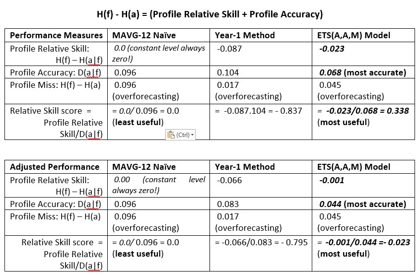
Profile Miss. A profile miss can be interpreted as a measure of ignorance about the forecast profile errors (FPE). The closer to zero the better, and the sign indicates over or underforecasting. The units are known as ‘nats’ (for natural logarithms).and ‘bits’ when using logarithms to the base 2 (e.g., climatology applications). I prefer ‘nats’ for lead-time demand forecasting. Thus, a forecast Profile Miss measures how different a forecast profile (or alphabet pattern) differs from a profile of actuals over a fixed horizon. For alphabet profiles, there is a measure of information H(a)that gives the information about the actual alphabet profile (AAP) and a measure H(f) that gives the information about a forecast alphabet profile (FAP). Hence, FAP Miss = H(f) – H(a):

Profile Accuracy. The accuracy of a forecast profile can be measured by a ‘distance’ measure between a forecast alphabet profile (FAP) and actual alphabet profile (AAP), given by the Kulback-Leibler divergence measure D(a,f): The D(a|f) measure is non-negative and is equal to zero if and only if a(i) = f(i), (i = 1,2, . .m). When D(a|f) = 0, the alphabet profiles overlap, or what we consider as 100% accuracy. 

L-Skill score. The profile accuracy measure D(a|f) can be decomposed into two components: (1) a forecast Profile Miss and (2) a forecast Profile relative skill measure. Thus, Profile Miss = Profile Relative Skill + Profile Accuracy. This means that accurately hitting a target involves both skill at aiming and scoring how far from the target the darts strike the dart board. You won’t win many medals by just accurately hitting any spot on the dartboard. And by becoming more accurate does not necessarily improve your standing in the process. You also need to improve your skill score in order to get closer to the real target.

The relative skill measure is in absolute value greater than zero, but does not include zero, unless the forecast profile errors are zero. The smaller, in absolute value, the better the relative skill. When a FAP is constant, as with the Croston methods, SES and MAVG-12 point forecasts, the relative skill is always equal to zero, meaning that with constant level methods a zero forecast profile miss is not possible. One good reason to scrap the MAVG-12 forecast or use it as a benchmark.

For the NaïveLT benchmark, we calculate Profile Accuracy = 0.052, which is better than MAVG-12 and almost as good as the ETS(A,A,M) model. Also, the Profile relative skill = – 0.014 is also better than MAVG-12 but not as effective as the ETS(A,A,M) model.

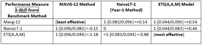
The Levenbach L-Skill score is the ratio of the Profile relative skill measure and the Profile accuracy. For the NaïveLT benchmark this is = -0.264, which is better than the ETS(A,A,M) model for the unadjusted data, but not after solving the data quality issue first. This makes NaïveLT benchmark a good benchmark for lead-time forecasting, as it requires no modeling assumptions. And data quality matters!

How the NaïveLT Benchmark Performs

In my practice, I have often seen demand planners start a forecast by taking last year’s actuals and applying a growth percentage to the Total and prorating that bias back to the individual periods. Sounds familiar? Here are the results. 

Hans Levenbach, PhD is Owner/CEO of Delphus, Inc and Executive Director, CPDF Professional Development Training and Certification Programs. Dr. Hans is the author of a new book (Change&Chance Embraced) on Demand Forecasting in the Supply Chain and created and conducts hands-on Professional Development Workshops on Demand Forecasting and Planning for multi-national supply chain companies worldwide. Hans is a Past President, Treasurer and former member of the Board of Directors of the International Institute of Forecasters.

Why You Need an Agile Consumer-Centric Demand Forecasting and Inventory Planning Process in a Disruptive Supply Chain Environment 4 Sep 2020, 3:26 pm

This is a foundational article about an algorithmic inferential modeling approach that supports an agile consumer-centric demand forecasting and inventory planning process without conventional normal (Gaussian) modeling assumptions. Conventional modeling assumptions may no longer work effectively in today’s disrupted supply chain environment, where unusual events and outliers tend to dominate demand history. Demand forecasting is becoming a greater challenge for demand and supply planning decision support systems designed with standard normal (Gaussian) modeling assumptions.

Regular and intermittent demand forecasting procedures are used for demand and inventory planning processes in practice, when 

• modeling product mix based on future patterns of demand at the item and store level
• selecting the most appropriate inventory control policy based on type of stocked item
• setting safety stock levels for SKUs at multiple locations

Intermittent demand (also known as sporadic demand) comes about when a product experiences several periods of zero demand. Often in these situations, when demand occurs it is small, and sometimes highly variable in size. In inventory control, the level of safety stock depends on the service level you select, on the replenishment lead time as well as the reliability of the forecast.

Step 1. Data Exploration as an Essential Quality Check in the Forecasting Process

Consumer demand-driven historical data, in the retail industry for example, are characterized to a large extent by trends (consumer demographics, business cycles) and seasonal patterns (consumer habits: economics). Before making any specific modeling assumptions, demand forecasters and planners should first examine data quality in the context of the new environment along with an exploratory data analysis (EDA) examination of the changing data characteristics and quality in demand history. if you want to achieve greater agility in forecasting for the entire supply chain, this preparatory step can be time consuming but is an essential undertaking, 

Looking for insight into data quality in this spreadsheet, you see that an expected seasonal peak for December 2016 seems to appear in the following month (Jan 2017). Interchanging the December with the January value appears to have a significant impact on the underlying seasonal variation, including uncertainty and other factors (compare ‘before’ in column 2 with ‘after’ in column 3 in the table below).

Also, May 2017 appears unusually weak, but we would call on domain experts to advise the forecaster on that unusual event. In any case, from a preliminary examination into the quality of the data, we see that consumer habit (an economic factor) may constitute about two-thirds of the total variation in the demand history (Above result obtained with a Two-way ANOVA w/o replication algorithm).

First Takeaway: “Bad data will beat a good forecaster every time” (Paraphrasing W. Edward Deming)

• Embrace Change & Chance by improving data quality through exploratory data analysis(EDA) as a preliminary step essential in creating agility in the demand forecasting and planning process.

For intermittent demand forecasting, on the other hand, it is necessary to examine the nature of the interdemand intervals and its relation to the distribution of non-zero demand sizes over a specified lead-time. The widely used Croston methods will under closer scrutiny point to flawed assumptions about the independence of zero intervals and demand volumes. Assumptions about Interval sizes and nonzero demand volumes should be reconciled in practice with real data, not just with simulated data.

Characterizing intermittent data with SIB models differs fundamentally from Croston-based methods in that a dependence of interval sizes on demand can be made explicit and can be validated with real data. The SIB modeling approach does not assume that intervals and demand sizes are independent or generated by conventional data-generating models.

The evidence of the dependence on interval durations for demand size can be explored by examining the frequency distribution of ‘lag time’ durations. I define a ”Lag-time” Zero­­ Interval LZI as the zero-interval duration preceding a nonzero demand size. In my previous LinkedIn article on SIB models for intermittent and regular demand forecasting, I focused on measurement error models for forecasting and evaluating intermittent demand volumes based on a dependence of an interval duration distribution. 

A Structured Inference Base (SIB) Model for Lead Time Demand

Step 2. Leadtime Demand Forecasting Needs a Specified Lead-time (Time Horizon) For lead-time demand forecasting with a fixed horizon, a location scale measurement error model can be created for assessing the effectiveness and accuracy of the demand forecasting process. The Profile Forecast Error (FPE) dataused in modeling the accuracy and performance of lead-time demand forecasts can be represented as the output of a measurement model: FPE = β + σ ɛ, in which β and σ are unknown parameters,  and the input ɛ is a measurement error with a known or assumed non-Gaussian distribution.

Keeping in mind the pervasive presence of outliers and unusual values in today’s real-world forecasting environment, I will henceforth shy away from the conventional normal distribution assumptions.  Rather, for error distribution assumptions, I will be referring to a flexible family of distributions, known as theExponential family. This is a rich family of distributions particularly suited for SIB modeling; it contains many familiar distributions including the normal (Gaussian) distribution, as well as distributions with thicker tails and skewness, so much more appropriate in today’s disruptive forecasting environment. These are some of the reasons I regard this article as foundational. However, by following a step-by-step development using a real-world data example and nothing more than arithmetic, some algebra and the logarithm, I hope that you can follow the process.

The SIB modeling approach is algorithmic and data-driven, in contrast to conventional data-generating models with normality assumptions. The measurement model for Forecast Profile Error (or Miss) = β + σ ɛ is known as a location scale measurement model because of its structure. The Forecast Profile Error (FPE) model shows that the FPE data result from a translation and scaling of an input measurement error ɛ. For the three forecasting approaches (judgment, method and model), used as examples, I display the FPE data below.

The forecast profile errors in the spreadsheet are calculated with the formula where a(i) are the components in the actual alphabet profile (AAP) and f(i) are the components in the forecast alphabet profile (FAP). These have been explained before in several previous articles available on my LinkedIn Profile and the my Delphus website blog.

The sums of the rows can be interpreted as a measure of information or ignorance about the forecast profile error. The closer to zero the better and the sign indicates over or underforecasting. In this example, the techniques are overforecasting. The units are known as ‘nats’ (for natural logarithms).

What Can Be Learned About the Measurement Process given the Forecast Profile Errors and the Observed Data?

Step 3. Setting Up the Model with Real Data

We can analyze the performance of a SIB model for lead-time forecasts as follows. In practice, we have multiple measurements of observed forecast profile errors (over a time horizon m = 12 in the spreadsheet example):

and where ɛ = {ɛ1, ɛ2, ɛ3, . . . ɛ12} are now 12 realizations of measurement errors from an assumed distribution in the Exponential family.

Step 4. A Critical Data Reduction Step

What information can we uncover about the forecasting process? Like a detective, we can explore a SIB model and find that, based on the observed data, there is a clue revealed now about the unknown, but realized measurement errors ɛ. This is evidence that will guide us to the next important SIB modeling step: It points to a decomposition of the measurement error distribution into two components: (1) a marginal distribution for the observed components and (2) a conditional distribution (based on the observed components) for the remaining unknown measurement error distribution, which depends on the parameters β and σ. So, what are these observed components of the error distribution that we uncover?

The insight or essential information is gleaned from the structure of the model and the recorded forecast profile error data. If we now select a suitable location measure m(.), and a scale measure s(.), we can make a calculation that yields important observables about the measurement process for each forecasting technique used. The SIB model shows, with some elementary algebraic manipulations, that the observables can be expressed in equations like this (using a 12-month lead-time):

That is, letting d = (d1, d2, … , d12) represent the left hand-side and right-hand side equations,we can reduce the SIB model to only two equations with two unknown variables m(ɛ) and s(ɛ) that represent the remaining unknown information in the measurement error model

Step 5. Conditioning on What You Know to be True

We do not need to go any further with details at this point. The conditional distribution (given the known d = (d1, d2, … , d12) for the variables m(ɛ) and s(ɛ) can be derived from the second equation using an assumed distribution for ɛ.

Using the selected location measure m(.), and a scale measure s(.), we can make a calculation that yields important observables about the measurement process for each method or model. If I select m(.) = L-Skill score as the location measure, the calculated L-Skill scores for the three approaches are obtained by summing the values on each row.

The L-Skill scores can range over the whole real line, the smaller the score in absolute value the better.Like the forecast profile accuracy measure D(a|f), the L-Skill score is zero if the actual and forecast alphabet profiles are identical. But, unlike the accuracy measure D(a|f), it can be shown that the L-Skill score will always be zero for constant level profiles, like MAVG-12.

The s(.) = Profile Accuracy D(a|f) divergences for the scale measure are found to be

We note that the 12 left-hand side equations named d(FPE) are equal to the right-hand side equations  d(ɛ). In the spreadsheet example for the 12 Lead-time demand values for Part #0174, d = d(FPE) = d(ɛ) is shown in the table. Then d = (d1, d2, … , d12), where we can now calculate

Step 6. Deriving Posterior Distributions for the Unknown Parameters β and σ Along with Posterior Prediction Limits and Likelihood Analyses

The derivations and formulae can be found in U of Toronto Professor D.A.S. Fraser’s 1979 book Inference and Linear Models, Chapter 2, and in his peer-reviewed journal articles dealing with statistical inference and likelihood methods. These are not mainstream results in modern statistical literature, but that does not diminish their value in practice.

Statistical inference refers to the theory, methods, and practice of forming judgments about the parameters of a population and the reliability of statistical relationships

These algorithms can be readily implemented in a modern computing environment, which was not the case more than four decades ago when I was first exposed to them. With normal (Gaussian) error distribution assumptions, there are closed form solutions (i.e. solvable in a mathematical analysis) that have a semblance to more familiar Bayesian inference solutions.

Step 7. Application to Inventory Planning

The SIB inferential analysis will yield a posterior distribution (conditional on the observed d) for the unknown parameters β and σ from which we can derive unique confidence bounds for β/σ (L-Skill score) and σ (Forecast Profile Accuracy). These confidence bounds will give us the service levels we require to set desired level of safety stock.

1.      For the ETS(A,A,M) model and data example, the reduced error distribution for location measure m(ɛ) and scale measure s(ɛ) is conditional on observed d = (d1, d2, … , d12):

·       Location component:            m(ɛ) = [m(FPE) – β]/ σ = [0.001 – β]/ σ

·       Scale component:                  s(ɛ) = s(FPE)/ σ = 0.044/ σ

2.      Define “Safety Factor” SF = √12 m(ɛ) /s(ɛ) = √12 {0.001– β 0}/ 0.044, where β 0 = max β under a selected contour boundary

Then,   β 0 = 0.001+ SF * 0.044/ √12 Is the desired level of safety stock for the service level you select.

Final Takeaway:

A data-driven non-Gaussian SIB modeling approach for lead-time demand forecasting is based on

• No independence assumptions made on demand size and demand interval distributions
• Non-normal (non-Gaussian) distributions assumed throughout the inference process.
• Using bootstrap resampling (MCMC) from a SIB model if the underlying empirical distributions are to be used
• Deriving posterior lead-time demand distributions with bootstrap sampling techniques
• Determining upper tail percentiles of a lead-time demand distribution from family of exponential distributions for lead-time demands or from empirical distributions

Hans Levenbach, PhD is Owner/CEO of Delphus, Inc and Executive Director, CPDF Professional Development Training and Certification Programs. Dr. Hans is the author of a new book (Change&Chance Embraced) on Demand Forecasting in the Supply Chain and created and conducts hands-on Professional Development Workshops on Demand Forecasting and Planning for multi-national supply chain companies worldwide. Hans is a Past President, Treasurer and former member of the Board of Directors of the International Institute of Forecasters.

The New L-Skill Score: An Objective Way to Assess the Accuracy and Effectiveness of a Lead-time Demand Forecasting Process 16 Aug 2020, 5:31 pm

Consumer demand-driven historical data are characterized to a large extent by seasonal patterns (consumer habits: economics) and trends (consumer demographics: population growth and migration). For the sample data, this can be readily shown using the ANOVA: Two Factor without Replication option in Excel Data Analysis Add-in. The data shown in the spreadsheet have an unusual value in January 2016. identified in the a previous post in my website blog; when adjusted it has a significant effect on the variation impacting seasonality (consumer habit) while reducing unknown variation.

Demand forecasting in today’s disrupted consumer demand-driven supply chain environment has become extremely challenging. For situations when – in pre new-normal times – demand occurs sporadically, the challenge becomes even greater. Intermittent data (also known as sporadic demand) comes about when a product experiences periods of zero demand. This has become more common during the pandemic supply chain, especially in the retail industry. The Levenbach L-Skill score, introduced here, is applicable in a ‘regular’ as well as intermittent lead-time demand forecasting process.

First Takeaway: Embrace change & chance by first improving data quality through exploratory data analysis (EDA). It is an essential preliminary step in improving forecasting performance.

A New Objective Approach to Lead-time Demand Forecasting Performance Evaluation

When assessing forecasting performance, standard measures of forecast accuracy can be distorted by a lack of robustness in normality (Gausianity) assumptions even in a ‘regular’ forecasting environment. In many situations, just a single outlier or a few unusual values in the underlying numbers making up the accuracy measure can make the result unrepresentative and misleading. The arithmetic mean, as a typical value representing an accuracy measure can ordinarily only be trusted as representative or typical when data are normally distributed (Gaussian iid). The arithmetic mean becomes a very poor measure of central tendency even with slightly non-Gaussian data (unusual values) or sprinkled with a few outliers.  This is not widely recognized among demand planners and commonly ignored in practice. Its impact on forecasting best practices needs to be more widely recognized among planners, managers and forecasting practitioners in supply chain organizations.

Imagine a situation in which you need to hit a target on a dartboard with twelve darts, each one representing a month of the year. Your darts may end up in a tight spot within three rings from the center. Your partner throws twelve darts striking within the first ring but somewhat scattered around the center of the dartboard. Who is the more effective dart thrower in this competition? It turns out that it depends not only how far the darts land from the center but also on the precision of the dart thrower.

In several recent posts on my LinkedIn Profile and this Delphus website blog, I laid out an information-theoretic approach to lead-time demand forecasting performance evaluation for both intermittent and regular demand. In the spreadsheet example, the twelve months starting September, 2016 were used as a holdout sample or training data set for forecasting with three methods: (1) the previous year’s twelve-month actuals (Year-1) as a benchmark forecast of the holdout data, (2) a trend/seasonal exponential smoothing model ETS(A,A,M), and (3) a twelve-month average of the previous year (MAVG-12). The twelve-month point forecasts over the fixed horizon of the holdout sample are called the Forecast Profile (FP). Previous results show that the three Mean Absolute Percentage Errors (MAPE) are about the same around 50%, not great but probably typical, especially at a SKU-location level.

We now want to examine the information-theoretic formulation in more detail in order to derive a skill score so that we can use it to assess the effectiveness of the forecasting process or the forecaster in terms of how much the method, model or forecaster contributed to the benefit of the overall forecasting process.

Creating an Alphabet Profile

For a given Forecast Profile FP, the Forecast Alphabet Profile FAP is a set of positive weights whose total sums to one. Thus, a Forecast Alphabet Profile is a set of m positive fractions FAP = [f₁ f₂, . . f_m] where each element f_i is defined by dividing each point forecast by the sum or Total of the forecasts over the horizon (here m = 12). This will give us fractions whose sum equals one.

Likewise, the Actual Alphabet Profile is AAP = [a₁, a₂, . . . a_m], where a_i is defined by dividing the Leadtime Total into each actual value and a Forecast Alphabet Profile FAP = [f₁ f₂, . . f_m], where f_i is defined by dividing the Leadtime Total into each forecast value. When you code a forecast profile FP into the corresponding alphabet profile FAP, you can see that the forecast pattern does not change.

For profile forecasting performance, we use a measure of information H, which has a number of interpretations in different application areas like climatology and machine learning. The information about the actual alphabet profile (AAP) is H(AAP) and the information about a forecast alphabet profile (FAP) is H(FAP), both entropy measures. There is also a measure of information H(a|f) about the FAP given we have the AAP information.

A Forecast Profile Error is defined by FPE _* a_i Ln a_i minus f_i Ln f_i, where Ln denotes the natural logarithm. Then summing the profile errors gives us the Forecast Profile Miss = H(f) – H(a):

The Accuracy D(a|f) of a forecast profile is defined as the Kullback-Leibler divergence measure D(a|f) = H(a|f) – H(a), where H(a|f) = – Sum (a_i Ln f_i ).

If we rewrite D(a|f) = [H(a|f) – H(f)] + [H(f) – H(a)], it results in a decomposition of profile accuracy into two components, namely the (1) Forecast Profile Miss = H(f) – H(a) and (2) a Relative Skill measure: H(f) – H(a|f), , the negative of the first bracketed term in the expression for D(a|f).

Another way of looking at this is using Forecast Profile Miss = Profile Accuracy + Relative Skill. In words, this means that accurately hitting the bullseye requires both skill at aiming and considering how far from the bullseye the darts strike the board.

The Relative Skill is in absolute value greater than zero, but does not include zero. The smaller, in absolute value, the better the Relative Skill and the more useful the method becomes. Remember, “All models are wrong, some are useful“, according the George Box. When a FAP is constant, as with the Croston methods, SES and MAVG-12 point forecasts, the Relative Skill = 0, meaning that with those methods, obtaining an (unbiased) Profile Bias of zero is clearly not possible. Hence, these methods are not useful for lead-time forecasting over fixed horizons. The M-competitions are examples of lead-time forecasting over fixed horizons.

For using forecasts on an ongoing basis, it might be useful to create an accuracy Skill score , defined by 1 – [D(a|f) / D(a|f*)] , where f* is a benchmark forecast, like the Year-1 Method, which is commonly used in practice. For lead-time forecasting applications, I call this the Levenbach L-Skill score. By tracking the L-Skill scores of the methods, models and judgmental overrides used in the forecasting process over time with, we have a means of tracking the effectiveness of forecasting methods.

Final Takeaway

In the context of a multistep-ahead forecasting process with a fixed horizon, we can assess the contribution of a method, model or forecaster in the performance of a forecasting process with the L-Skill score. In theory, statistical forecasting models are designed to be unbiased, but that theoretical consideration may not be valid in practice, particularly for ‘fixed horizon’ lead-time demand forecasting. Moreover, multiple one-step ahead forecasts have little practical value in lead-time demand forecasting as the lead-time is the ‘frozen’ time window in which operational changes can usually not be made.

Try it out on some of your own data and see for yourself what biases and performance issues you have in your lead-time demand forecasts and give me some of your comments in the meantime. I think it depends on the context and application, so be as specific as you can. Let me know if you can share your data and findings.

Hans Levenbach, PhD is Executive Director, CPDF Professional Development Training and Certification Programs. Dr. Hans is the author of a new book (Change&Chance Embraced) on Demand Forecasting in the Supply Chain and created and conducts hands-on Professional Development Workshops on Demand Forecasting and Planning for multi-national supply chain companies worldwide. Hans is a Past President, Treasurer and former member of the Board of Directors of the International Institute of Forecasters.

Embracing Change and Chance. The examination of an forecasting process would not be complete until we consider the performance of the forecasting process or forecasters. This new Levenbach L-skill score measure of performance is included in my latest revision of the paperback available on Amazon (https://amzn.to/2HTAU3l).

How You Can Determine the Bias in a Leadtime Demand Forecast 16 Aug 2020, 4:01 pm

In a global pandemic environment, lead-time demand forecasts become increasingly important in planning production capacities, managing product portfolios, and controlling inventory stock outs in the supply chain. In inventory planning, for example, the lead time demand is the total demand between the present and the anticipated time for the delivery after the next one if a reorder is made now to replenish the inventory. This delay is called the lead-time. Since lead time demand is a future demand (not yet observed), this needs to be forecasted. While models are designed to produce unbiased forecasts, how can we determine whether forecasts are biased or not over the desired lead-time. This means that individual point forecasts as well as the lead-time total can be biased.

In a previous article, I introduced a measure of accuracy for lead time demand forecasts that does not become unusable with intermittent demand, like the widely used Mean Absolutes Percentage Error (MAPE). The MAPE can be a seriously flawed accuracy measure, in general, and not just with zero demand occurrences. In another articleand website blog, I posted a new way you can forecast intermittent demand when the assumption of independence between intervals and nonzero demands is not plausible, making the Croston methods inappropriate. I use information-theoretic concepts, like KL Divergence, in this new approach to intermittent demand forecasting,

Creating the Actual Holdout Sample and Forecast Profiles

We start by defining a multi-step ahead or lead-time forecast as a Forecast Profile (FP). A forecast profile can be created by a model, a method, or informed judgment. The forecast profile of an m-step-ahead forecast makes up a sequence FP = { FP(1), FP(2), . . . , FP(m) } of point forecasts over the lead-time horizon. For example, the point forecasts can be hourly, daily, weekly or more aggregated time buckets.

I have been using real-world monthly holdout (training) data starting at time t = T and ending at time t = T + m, where m = 12. Typically, lead-times could be 2 months to 6 months or more, the time for an order to reach an inventory warehouse from the manufacturing plant. For operational and budget planning, the time horizon might be 12 months to 18 months. This 12-month pattern of point forecasts is called a Forecast Profile.

At the end of the forecast horizon or planning cycle, we can determine a corresponding Actual Profile AP ={ AP(1), AP(2), . . . , AP(m) } of actuals to compare with FP for an accuracy performance assessment. Familiar methods include the Mean Absolute Percentage Error (MAPE). The problem, in case of intermittent demand, is that some AP values can be zero, which leads to undefined terms in the MAPE.

We are approaching forecasting performance by considering the bias in the Forecast Profile using information-theoretic concepts of accuracy.

Coding a Profile into an Alphabet Profile

For a given Profile, the Alphabet Profile is a set of positive weights whose sum is one. That is, a Forecast Alphabet Profile is FAP = {f(1) f(2), . . . f(m)}, where f(i)= FP(i)/Sum FP(i). Likewise, the Actual Alphabet Profile is AAP = {a(1), a(2), . . . a(m)], where a(i) = AP(i)/Sum AP(i). The alphabet profiles are defined by:

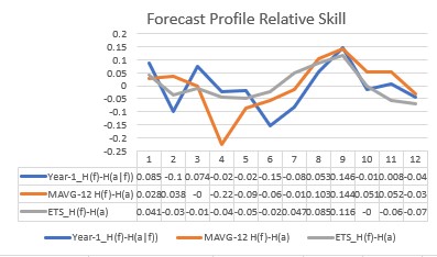
But, what about the real data profiles FP and AP shown in the lower frame below ? For the spreadsheet data example, the two forecasts show different FP profiles.

When you code a forecast profile FP into the corresponding alphabet profile FAP, you can see that the demand pattern does not change for the Year-1 method, and ETS(AAM) model. (The models were explained in the previous articles)

In practice, the performance of a forecasting process leads us to make use of various metrics that need to be clearly defined first, so that in practice, planners and managers do not talk ‘apples and oranges’ and possibly misinterpret them. The alphabet profile is necessary in the construction of a ‘Statistical Bias’ measure I am proposing for lead-time demand forecasting for both regular and intermittent demand.

The relative entropy or divergence measure is used as a performance measure in various applications in meteorology, neuroscience and machine learning. I use it here as a measure of how a forecast profile diverges from the actual data profile. An accuracy measure for the forecast alphabet profile (FAP) is given by a Kullback-Leibler divergence measure D(a|f), which can be readily calculated in a spreadsheet.

For a perfect forecast, a(i) = f(i), for all i, so that D(a|f) = 0 and (shown below) FAP Miss = 0. Since D(a|f) can be shown to be greater than or equal to zero, this means that for a perfect forecast, zero is the best you can achieve. In all other cases, accuracy measure D(a|f) will be greater than zero. Thus, with a perfect forecast the coded alphabet profiles FAP and AAP are identical and overlap with no bias.

Now, a Forecast Alphabet Profile Miss or Bias is shown in the formula above . In information-theoretic terms the summation terms are known as ‘entropies’ and will be interpreted as information about AAP and FAP, respectively. The Miss or Bias is the difference between the two entropies. The unit of measurement is ‘nats’ because I am using natural logarithms in the formula or “logarithms to the base e”. In Information theory and climatology applications, it is more common to use “logarithms to the base 2”, so the units of measurement are then ‘bits’. The meaning of bias remains the same. By substituting for a(i)and f(i) in the logarithm terms in the above formula, we can show that

With a perfect forecast, the AP pattern and FP patterns are identical but do not overlap because the patterns do not have the same lead time totals. The profiles would be parallel but thus show a bias. Thus, the formula below is the desired bias term between FAP Miss and FP Miss, shown in the spreadsheet above in the last column (in bold). You can verify that when the total lead time forecast = total lead time actuals, then ln (1) = 0 and the Bias = 0. In the holdout sample, ETS model had the largest overall Bias; however, it had fewer and smaller swings of over and under forecasting in the point forecasts, so point forecast bias and lead-time demand total bias are both important. 

But, This is Not All!

In a follow-up article, I will show that further examination of these information entropies, will lead to a Skill Score we can use to measure the performance of the forecaster in terms of how much the forecaster skill benefitted the forecasting process! Is it better or worse to have large over and under forecasting swings than it is to show an overall under forecasting bias of the total lead-time forecast? Hopefully, the Skill Score with give additional insight into the lead-time demand forecasting performance issue.

Try it out on your own data and see for yourself what biases you have in your lead-time demand forecasts and give me some of your comments in the meantime. I think it depends on the context and application, so be as specific as you can.

Hans Levenbach, PhD is Executive Director, CPDF Professional Development Training and Certification Programs. Dr. Hans is author of a new book (Change&Chance Embraced) on Demand Forecasting in the Supply Chainand created and conducts hands-on Professional Development Workshops on Demand Forecasting and Planning for multi-national supply chain companies worldwide. Hans is a Past President, Treasurer and former member of the Board of Directors of the International Institute of Forecasters. He is Owner/Manager of the LinkedIn groups

(1) Demand Forecaster Training and Certification, Blended Learning, Predictive Visualization, and

(2) New Product Forecasting and Innovation Planning, Cognitive Modeling, Predictive Visualization.

How You Can Improve Forecasting Performance with the MAPE by Finding and Fixing Data Quality Issues in Your Demand History 11 Jul 2020, 5:12 pm

In a recent article entitled Improving Forecasting Performance with Intermittent Data – A New Way of Scoring Performance, I gave some insight into why the MAPE (Mean Absolute Percentage Error) can be a seriously flawed accuracy measure. Aside from intermittency. when demand has zeros and APEs (Absolute Percentage Errors) are undefined, there are often unusual values in the APEs that distort the average. I showed that there is a remedy that you can apply by considering the MdAPE (Median Absolute Percentage Error) or the HBB TAPE (Typical Absolute Percentage Error) as a more typical summary than the average. The HBB TAPE metric was introduced in my LinkedIn post and is also described in my book Change&Chance Embraced (p. 97) dealing with smarter, agile demand forecasting practices for the Supply Chain. I have also used it in facilitating CPDF professional development workshops (see the CPDF Workshop Manual, p. 188., available on Amazon). I have also placed my articles on my website blog.

In this article, I show how the difference between the MAPE and MdAPE can lead to insights into why the MAPE has been so misleading as an accuracy measure. The MAPE appears to be commonly provided in demand planning software without reservation. 

In this spreadsheet example, the twelve months starting September, 2016 (row 11) was taken as a holdout sample or training data set for forecasting with three methods: (1) the previous year’s twelve-month actuals (Year-1), (2) a trend/seasonal exponential smoothing model ETS(AAM), and (3) a twelve-month average of the previous year (MAVG-12). The twelve-month forecasts in the holdout sample are called Forecast Profiles (FP). The results ((left panel, row 34) show that the three MAPEs for the twelve months are about the same around 50%, not great but probably typical, at a SKU-location level. 

However, when you calculate the MdAPEs (left panel, row 35) for these data, you get a strikingly different and better result for a summary performance of the three forecast profiles, Year-1, ETS(AAM) and MAVG-12, as follows: Year-1 (41%), ETS(AAM) (25%) and MAVG-12 (32%).

Using Gaussian Arithmetic is Not Always a Best Practice

What’s the story here? As they say, the information is the in the DATA. There maybe an outlying or unusual value in the APEs that distorts averaging with the arithmetic mean (“Gaussian arithmetic”). Is the simple average MAVG-12 really more accurate than the Year-1 forecast profile and only slightly less valuable than the ETS model forecast profile?

The takeaway here is that you need to ALWAYS be able to examine the underlying data for anomalies that commonly distort or disguise results. Many software systems may not always give you that flexibility, however.

Add alt text

When you examine the historical data more closely with an ETS model, you can see that the data are seasonal with a seasonal peak in December (not surprisingly) and a seasonal trough in July.

Now, the peak month in 2016 holdout data in the spreadsheet (cell F11) does not appear in December (= 49786), as expected, but rather the following month, January 2017 (=75069). This is not credible, so for the sake of model integrity and stability in performance measurement, the two data values are switched in the spreadsheet, and the MAPEs and MdAPEs recalculated

I want to capture the change in the MAPE as the holdout year progresses. So, I calculate a rolling MAPE starting in period 5 (using periods 1-5, etc.) of the holdout period and continuing until end of the holdout period. The chart to the right of the table (top panel) summarizes the results graphically. There is no clear distinction between the performance of a level profile (MAVG-12) and the ETS(AAM) profile in the unadjusted MAPEs. However, with the December anomaly found and fixed, it becomes clear with the MdAPEs that the ETS(AAM) forecast profile clearly outperformed the other two during this period (lower panel). The MdAPE is outlier-resistant and a gives a better picture of a typical accuracy, while the MAPE never can when there are outliers and unusual values (even one or two!).

Another takeaway: It should not be a best practice for demand planners to rely on MAPEs alone.

As I pointed out before, this forecast profile analysis with MAPEs is not appropriate with intermittent lead-time demand data. In a follow-up article, I will again use a more appropriate information-theoretic approach to forecast accuracy measurement, which is valid for both regular and intermittent demand forecasting. Moreover, you will see that the approach allows for direct comparisons between the forecasting performance at the SKU level any any corresponding summary level (product family, brand, etc.), because of the use of comparable alphabet profiles.

When NOT to Use the Croston Method for Intermittent Demand Forecasting 17 Jun 2020, 8:54 pm

In an earlier article on Forecasting with Intermittent Demand, a reader asked me whether my (Structured Inference Base) SIB approach for intermittent demand modeling was applicable to daily and weekly data, as well as the monthly example I gave. It is, and could in fact work for any intermittent time series.

The point of this article is that the Croston method, while widely implemented for forecasting intermittent demand, may not be applicable in real-world data applications. The reason is that the underlying assumptions about the independence of intervals and demand volumes may not be valid in practice. The method and its variants essentially take interval durations and nonzero demand volumes as separate data series for forecast modeling purposes.

When you start looking at real data, you may find that the demand volumes can depend on the interval durations, as I will now demonstrate with a series of 52 intermittent weekly demand (ID) data.

Intermittent data  (also known as sporadic demand) comes about when a product experiences several periods of zero demand. This has become more common during the pandemic supply chain disruptions, especially in the retail industry. Forecasting intermittent demand occurs in practice, when

1. modeling product mix based on future patterns of demand at the item and ship-to location level
2.  selecting the most appropriate inventory control policy based on type of stocked item
3. setting safety stock levels for SKUs at multiple locations

Often in these situations, when demand occurs, it is small, and sometimes highly variable in size. For example, the level of safety stock depends on the service level you select, on the replenishment lead time and on the reliability of the forecast.

Here, I will show that a mutual information measure I(ID, LZI) gives the error in assuming the independence of nonzero intermittent demand volumes (ID) and the zero interval durations (LZI). This formula is widely used in information theory and climatology applications and can be applied in intermittent demand applications, as well. In the mutual information formula (and the Kullback-Leibler divergence measure KL), P represents a discrete probability distribution; that is, like positive weights, whose sum is one.

Let us try to validate this with some real data. You can follow the procedure with the spreadsheet below. The intermittent demand series is depicted in Column A. There are 38 nonzero demand volumes and 18 zeroes of duration 1 and 2, giving a total of 52 weeks.

In using the mutual information formula, P(ID) is the Intermittent Demand volume alphabet profile (Col D); P(LZI) is the Lagtime Zero Interval alphabet profile (Col C); P(ID, LZI) is the Joint alphabet profile (Col B), denoted by JOINT in the spreadsheet. P(.) is a marginal alphabet profile in the formula.

In our use of the formula, P defines an alphabet profile, which is coded from the original data into numbers between 0 and 1, summing up to 1. Thus, to obtain the alphabet profile P(ID) in column D, we divide the sum of the ID history (=73) into each nonzero demand value in Col A. These 38 ratios sum to one. You can see on the graphs below that the original history profile and the corresponding alphabet profile have the same pattern and differ only by the scale on the y-axis. 

The zeros for LZI in the dataset are the same number, so the alphabet profile P(LZI) in column C is a set of 14 constant numbers (=1/14), also summing to one.

In the mutual information formula, there is a joint alphabet profile P(ID, LZI) that needs to be created (Col B). In our formulation of the relationship between intervals and demand volumes, we postulate that each interval is followed by a nonzero demand. We call the intervals LZI, for Lagtime Zero Interval. In this data set, there are 3 two-zero intervals, 8 one-zero intervals, and 27 no-zero intervals (27= 38-11). In this way, there is an LZI value associated with each demand volume. This process creates a conditional distribution of demand volumes dependent on the LZI variable.

The joint alphabet profile is obtained by multiplying each value in Col D by its corresponding weight in the LZI_0, LZI_1, LZI_2 distribution (= 0.78082, 0.16438, 0.05479). The results are added up and subtracted from 1. That difference is apportioned to the remaining 14 zeros in Col B ( 0.03201 = 0.44814/14).

The Accuracy of the Independence Assumption

It the demand volumes and interval durations are independent the mutual information measure I(ID, LZI) = 0. If I(ID, LZI) = 0, it implies independence. It can be shown that the measure I(ID, LZI) ≥ 0, so that a positive value of I(ID, LZI) indicates a lack of independence or association. In this example, I(ID, LZI) = 0.56, suggesting a lack of independence. (row 56: = Col E – Col F – Col G). You will have to run many of your own examples to establish a range away from zero to test the assumption.

How to Measure Leadtime Demand Accuracy for Forecast Profiles – An Information-theoretic Approach 17 Jun 2020, 8:46 pm

Demand forecasting and performance evaluation in today’s disrupted consumer demand-driven supply chain environment has become an extremely challenging discipline for business planners to master. For instance, current forecasting performance metrics for intermittent demand have shortcomings that are not easily overcome. In particular, the widely used Mean Absolute Percentage Error (MAPE) metric is unusable in this context when no demand is encountered. To embrace more agile and reliable approaches, I will consider a new metric for multi-step ahead forecasts with fixed horizons (e.g. Leadtime demand forecasts) by using relative entropy measures from information theory.

Before dealing with intermittent demand forecasting applications, I will examine a lead-time demand forecasting example without intermittency first. The approach will be equally applicable. I have added the notation in the spreadsheet, so you can follow this with your own data.

In the dataset, the holdout data (in italics) are shown in the row for year 2016. A fiscal, budget or planning year does not necessarily have to start in January, so lead-time or forecasting cycle totals are shown also, as we will be using them in our calculations. For a twelve-month holdout sample, we have created three forecasts by judgment, method and model:

For a judgment forecast, we will assume last year actuals as the forecast for the next year. This forecast profile is Year-1 FP. For a method, we use the constant MAVG_12 FP, which is simply the average of previous 12-month history. The MAVG12 method has a level profile.

The model forecast is based on the ETS (A,A,M) which has a local level, multiplicative seasonal forecast profile and is a State Space forecasting model described in Chapter 8 of my book. The model was selected in automatic mode since the profile is a deterministic trend/seasonal profile.

We start by defining a multi-step ahead forecast with a fixed horizon (e.g. lead-time forecast) as a Forecast Profile (FP). A forecast profile can be created by a model, a method, or informed judgment. The forecast profile of a m-step-ahead forecasts makes up a sequence FP = { FP(1), FP(2), . . . , FP(m) }. For our example, we will assume that the forecasts are monthly starting at time t = T and ending at time t = T + m, where m = 12. Typically, lead-times could be 2 months to 6 months or more, the time for an order to reach an inventory warehouse. For operational and budget planning, the time horizon might be 12 months. This 12-month pattern is called a Forecast Profile.

At the end of the forecast horizon or planning cycle, there is a corresponding Actual Profile AP ={ AP(1), AP(2), . . . , AP(m) } to compare with FP for an accuracy assessment. Familiar methods include the Mean Absolute Percentage Error (MAPE). The problem, in case of intermittent demand, is that some AP values can be zero, which leads to undefined terms in the MAPE.

We are going to evaluate forecasting performance by considering the information in the Forecast Profile using information-theoretic measures. Then we can assess how the forecast profile diverges from the pattern or profile in the actuals. 

Coding a Profile Into an Alphabet Profile

For a given Profile, the Alphabet Profile is a set of weights whose sum is one. That is, a Forecast Alphabet Profile is FAP = {f1, f2, . . . fm ], where fi = FP (i)/ . In other words, we simply divide each forecast by the sum of the forecasts over the horizon. This will give us fractions whose sum equals one. The Actual Alphabet Profile is AAP = {a1, a2, . . . am], where ai is the ratio of the actual to the Total Leadtime actuals. When we compare a profile with the corresponding alphabet profile, we note that the pattern does not change.

An Information-theoretic Accuracy Measure of Forecast Profile Performance

The performance of the process that created the Forecast Profile is of interest because we will come up with a ‘distance’ metric between the Forecast Profile and Actual Profile that has its basis in Information Theory. We notice in the graphs that the alphabet profilehas the same pattern as the corresponding source profile from which it was created. The alphabet profile is necessary in the construction of the ‘distance’ metric.

The relative entropy or divergence measure is used as a performance measure in various applications in meteorology, neuroscience and machine learning. I use it here as a measure of how one forecast profile diverges from another profile. A performance measure for the forecast alphabet profile (FAP) is given by a Kullback-Leibler divergence measure, which can be interpreted as a measure of dissimilarity or ‘distance’ between the actual alphabet AAP and forecast alphabet FAP profiles. The measure, known as the Kullback-Leibler divergence, is non-negative and is equal to zero if and only if ai = fi (I = 1,2, . . m). This happens when the alphabet profiles overlap, or what we might consider as 100% accuracy.

A Decomposition of the Divergence Measure D(AAP, FAP)

The MAVG_12 FP is level, as is the Naïve_1 (NF1) FP and simple exponential smoothing (SES) FP. In these cases,

where m = 12. The first term is known as the entropy H of AAP and is a measure of the information in AAP. Hence, D(AAP, FAP) = ln (12) – H (AAP), in this example.

For a single forecast, Actual (A) minus Forecast (F) is the accuracy of the forecast, so D(AAP, FAP) can be viewed as a measure of accuracy for a single Actual (AP) and Forecast (FP) profile. That is how I propose D(AAP, FAP) can be used for assessing the performance of multi-step-ahead and lead-time demand forecasts.

I am unaware of where this accuracy measure has been previously used in the forecasting literature or used in demand forecasting software or applications. Someone might wish to bring this to my attention.

In a previous blog on my website and a LinkedIn article, I gave a spreadsheet example of the Forecast Profile Performance (FPP) index to measure intermittent demand forecast accuracy. I invite you to join the LinkedIn groups I manage and share your thoughts and practical experiences with intermittent data and smarter demand forecasting in the supply chain. Feel free to send me the details of your findings, including the underlying data used without identifying descriptions, so I can continue to test and validate the process for intermittent data.

A New Way to Monitor Accuracy of Intermittent Lead-time Demand Forecasts: The Forecast Profile Performance (FPP) Index 17 Jun 2020, 8:41 pm

Intermittency in demand forecasting is a well-known and challenging problem for sales, inventory and operations planners, especially in today’s global supply chain environment. Intermittent demand for a product or service appears sporadically with lots of zero values, and outliers in the demand data. As a result, accuracy of forecasts suffers, and how to measure and monitor performance has become more critical for business planners and managers to understand. The conventional MAPE (Mean Absolute Percentage Error) measure is inadequate and inappropriate to use with intermittency because of divisions by zero in the formula lead to undefined quantities.

In a previous article, I introduced a new approach, which can be more useful and practical than a MAPE in dealing with inventory lead-times , financial budget planning, and sales & operations (S&OP) forecasting. What these applications have in common are the multi-step ahead forecasts, whose accuracy needs to be assessed on a periodic basis. I will call this new approach the Forecast Profile Performance (FPP) process.

A Smarter Way to Deal with Intermittency in Demand Forecasting

For the past four to five decades, the conventional approach in dealing with intermittency has been based on the assumption that interdemand intervals and the nonzero demand events are independent. This is the logic behind the Croston method and its various modifications. But, when you start looking at real data in an application, you discover that this may not be valid.

This new approach examines the data in two stages. First, we observe that each demand event is preceded by an interdemand interval or duration. Thus, given a duration, we can assume that a demand event follows. In a regular demand history, each demand event is preceded by an interval of zero duration. Under this assumption, non-zero Intermittent Demand events ID* are dependent on ‘Lagtime’ Zero Interval durations LZI. The LZI distribution for our spreadsheet example is shown in the left frame. In the right frame, we show the conditional distribution for the ID* given the three LZI durations. They are not the same hence it would not be advisable to assume that they are. 

When forecasting ID* for an inventory safety stock setting, for example, it will be necessary to consider each of the conditional distributions separately. In the spreadsheet above, I have created three forecasts for the 2017 holdout sample. Forecast F1 is a level naïve forecast with 304 units per month. For ease of comparisons, I have assumed that annual totals are the same as the holdout sample. In practice, this would not necessarily be true. The same is assumed for Forecasts F2 and F3. so that comparisons of forecast profiles are the primary focus. In practice, the effect of a ‘bias correction’, if multi-step forecast totals differ, should also be considered, However, consideration of the independence assumption is a fundamental difference between a Croston method and this one.

Step 1. Creating Duration Forecasts

When creating forecasts, we first need to forecast the durations. This should be done by sampling the empirical or assumed LZI distribution. In our spreadsheet, LZI_0 intervals occur more frequently than the other two and the LZI_1 and LZI_2 intervals occur with about the same frequency. Then, based on the LZI in the forecast, a forecast of ID* should be made from the data the LZI it depends on. An example of this process is given in an earlier post and on the Delphus website.  

After a forecasting cycle, is completed and the actuals are known, both the LZI distribution and the conditional ID* distribution need to be updated before the next forecasting cycle, so the distributions can be kept current.

Step 2. Creating the Alphabet Distributions

Depending on your choice of a Structured Inference Base (SIB) model for intermittent demand ID* (or the natural log transformed intermittent demand Ln ID*), alphabet profiles need to be coded for the actuals and the forecasts from the (conditional) demand event distributions for each of the durations LZI_0 in column C, LZI_1 in column F, and LZI_2 in column I. Note that the sum of the weights in an alphabet profile add up to one.

For the data spreadsheet we need also the add the alphabet weights associate with the duration distribution. This is done by multiplying the conditional alphabet weights by the weights in the (marginal) duration distribution LZI_0 (= 0.4545), LZI_1 (= 0.2727), and LZI_2 (= 0.2727). These coded alphabet weights can be found in columns D, G, and J, respectively. Note that the sum of the three weights in the combined alphabet profiles add up to 1.

Step 3. Measuring the Performance of Intermittent Demand Profiles

In a previous article on LinkedIn as well as my website blogs, I introduced a measure of performance for intermittent demand forecasting that does not have the undefined terms problem arising from intermittency. It is based on the Kullback-Leibler divergence or dissimilarity measure from Information Theory applications.

where a(i ) (i = 1,2, …, m) are the components of the Actuals Alphabet Profile (AAP) and f(i) (i = 1,2, …, m) are the components of the Forecast Alphabet Profile (FAP), shown in the spreadsheet below. In the forecast, the lead-time, budget cycle, or demand plan is the horizon m.

Step 4. Creating a Forecast Profile Performance (FPP) Index

The alphabet profile for the actuals (AAP) is shown in the top line of the spreadsheet above. The alphabet profiles for the forecasts (FAP) are shown in the second, fourth, and sixth lines in the spreadsheet. The calculations for the D(a|f) divergence measure are shown in the third, fifth, and seventh lines with the D(a|f) results shown in bold. They are 22%, 40%, and 16%. respectively, for forecasts F1, F2, and F3. It can be shown that D(a, f) is non-negative and equal to zero, if and only if, the FAP = AAP, for every element in the alphabet profile. Hence, F3 is the most accurate profile followed by F1 and F2. This should not be interpreted to mean that F3 has the best model. However, it does suggest that the F3 model has the best multi-step ahead forecast pattern of the actuals. One should monitor D(a, f) for multiple forecasting cycles, as trend-seasonal patterns can change for monthly data, in this instance.

FPP (f) index = 100 + D(a|f)

We can create a Forecast Profile Performance index by adding 100 to D(a f), so that 100 is the base for the most accurate possible profile.

Step 5. Monitoring a FPP index.

The FPP index needs to be charted for every forecasting cycle, much like a quality control chart in manufacturing. One way of creating bounds for the index is to depict three horizontal bars (green, amber and red), where the lowest bar, starting at 100, is the limit for an acceptable accurate profile, the middle bar for profiles to be reviewed, and the red bar for unacceptable performance. The criteria for the bounds should all be based on downstream factors developed from your particular environment and application.

I invite you to share your thoughts and practical experiences with intermittent data and smarter demand forecasting in the supply chain. Feel free to send me the details of your findings, including the underlying data used without identifying descriptions, so I can continue to test and validate the process for intermittent data.

Improving Forecasting Performance for intermittent data: A New Measurement Approach 17 Jun 2020, 8:31 pm

With today’s disruptions in global supply chains as a result of the coronavirus pandemic, intermittent sales volumes, shipments and service parts inventory levels are becoming more common across many industries, especially in retail. Intermittent demand forecasting for a product or service with sporadically scattered zero values in the demand data is a challenging problem. As a result, demand forecasting for a modern consumer demand-driven supply chain organization is becoming a more vital discipline for business planners to master.

In this article, I introduce a new way of measuring forecasting performance that does not have the shortcomings of the widely used Mean Absolute Percentage Error (MAPE) metric in this context. To keep matters simpler, I will introduce the new metric using regular trend/seasonal data. An example with intermittent data will follow this article.

Before dealing with the intermittent demand case, we will examine a forecast profile example without intermittency, something smarter to start with if you are considering to add this to your toolkit and want to test the methodology with your own data. I have added the notation on the spreadsheet, so you can follow this example with your own data.

In the spreadsheet dataset, the holdout sample (in italics) is shown in the row for year 2016. A fiscal, budget or planning year does not necessarily have to start in January, so lead-time or forecasting cycle totals are shown also, as we will be using them in our calculations.

Step 1. Preliminaries. What is a Forecast Profile?

We start with a little notation, so that you can test and follow the steps in a spreadsheet environment for yourself. Suppose we need to create forecasts over a time horizon m , like a leadtime or annual planning or budget cycle. These multi-step ahead forecasts, created by a model, method or judgment. make up a sequence FP = { FP(1), FP(2), . . . , FP(m) }. For our example, we will assume that the forecasts are monthly starting at time t = T and ending at time t = T + m. Typically, lead-times could be 2 months to 6 months, the time for an order to reach an inventory warehouse. For operational and budget planning, the time horizon might be 12 months. We call this pattern a Forecast Profile. At the end of the forecast horizon or planning cycle, we will have a corresponding Actual Profile AP ={ AP(1), AP(2), . . . , AP(m) } to compare with FP. Familiar methods include the calculation of the Mean Absolute Percentage Error (MAPE). In the case of intermittent demand, some actuals are zero, which leads to undefined terms in the MAPE.

Step 2. Coding a Profile Into an Alphabet Profile

We are interested in evaluating forecasting performance or “accuracy” by considering the information in the Forecast Profile and see how different that is from the information in the profile of the actuals.

Add alt text

The performance of the process that created the Forecast Profile is of interest because we will come up with a ‘distance’ metric between the Forecast Profile and Actual Profile that has its basis in Information Theory. As you can see in the graphs, the alphabet Profile has the same pattern as the historical Profile from which it was created, but is necessary in the construction of the ‘distance’ metric.

For a given profile, the alphabet profile is a set of weights whose sum is one. That is, a Forecast Alphabet Profile is FAP = {f1, f2, . . . fm ], where fi is calculated by simply dividing each forecast by the sum of the forecasts over the forecast horizon. This will give us fractions whose sum is one. The Actual Alphabet Profile is AAP = {a1, a2, . . . am], where ai is obtained by dividing each actual by the sum of the actuals over the forecast horizon. When you compare a historical profile with the corresponding alphabet profile, the pattern does not change.

Step 3. A Forecast Performance Metric for Multi-Step Ahead Forecasts (Forecast Profiles).

The ‘relative entropy’ or ‘divergence; measure are being used as performance measures in various applications in meteorology, neuroscience and machine learning. I use it here as a measure of how one forecast profile is different from another profile. We wil first define the entropy H(.) as a way of measuring the amount of information in the alphabet profiles, as follows:

Thus, – H(FAP) can be interpreted as the amount of information associated with the Forecast Alphabet Profile. Similarly, – H(AAP) is interpreted as the amount of information associated with the Actual Alphabet Profile. Both quantities are greater than or equal to zero and have units of measurement called ‘nats’ (for natural logarithm). If you use logarithms to the base 2, the units are in ‘bits’, something that might have a more familiar ring to it.

A Performance Measure for Forecast Profiles

A performance measure for the forecast alphabet profile (FAP) is given by a divergence measure

This can be interpreted as a measure of dissimilarity or ‘distance’ between the actual and forecast alphabet profiles. The measure is non-negative and is equal to zero if and only if ai = fi (i = 1,2, . . m). This happens when the alphabet profiles overlap, or what we would call 100% accuracy. I am unaware of where this measure has been previously proposed in the forecasting literature or actually implemented in demand forecasting applications.

It should be pointed out that this measure is asymmetrical, in that D(a, f) is not equal to D(f, a). That should be evident from the formula. Also, the alphabet profiles are not discrete probability distributions, so some interpretations normally attributed to this divergence measure may not be applicable. This divergence measure is known as the Kullback-Leibler divergence.

Step 4. Looking at Divergence Measures with Real Data

For the twelve-month holdout sample, we have created three forecasts by judgment, method and model:

1. For a judgment forecast, we will assume last year actuals as the forecast for the next year. This forecast profile is Year-1 FP. 
2. For a naive method, we use the MAVG12 forecast, which is simply the average of a previous 12-month history. The MAVG12 method has a level profile.
3. The model forecast is based on the ETS (A,A,M) model which has a local level and multiplicative seasonal forecast profile. The model was selected in an automatic mode since the profile is deterministic. The State Space ETS Exponential Smoothing Models are described in Chapter 8 of my book.

Calculating Alphabet Profiles and the Divergence Measure

The determination of the alphabet profiles are shown in the spreadsheet along with the divergence calculations. The divergence measurements are shown in bold. Since matching profiles result in the lower bound of zero, the closer to zero the better. This would suggest that the ETS forecast is the least divergent (of the three profiles or different) from the actuals.

A Comparison With the Traditional Accuracy Measurement MAPE

If we compare the results with a Mean Absolute Percentage Error (MAPE) calculation for the holdout sample, we see that the ETS model has the best MAPE. This is not to say that it will always be the case, but at least the results are consistent with the divergence measure. 

However, there seems to be a more serious issue with the MAPE that I have written about previously in an article here, in that the MAPE is not a reliable representative or typical value for the APEs when there are unusual or zero values in the actuals. If you also calculate the Median APE (MdAPE), however, you will note that the underlying APEs are skewed with thicker tails that prescribed by a normal distribution. This has not been adequately noted by forecast practitioners that the underlying distribution of the data used in a calculation with the arithmetic mean is critical. Forecasters should always quote the MdAPE with the MAPE to avoid loss of credibility.

There is an outlier-resistant measure you can use to validate the MAPE; it is called HBB TAPE (Typical Absolute Percentage Error) for which I have shown an example in my book, an article here on LinkedIn, and a blog on my website.

Hans Levenbach, PhD is Executive Director, CPDF Professional Development Training and Certification Programs. Dr. Hans created and conducts hands-on Professional Development Workshops on Demand Forecasting and Planning for multi-national supply chain companies worldwide. Hans is a Past President, Treasurer and former member of the Board of Directors of the International Institute of Forecasters. He is group manager of the LinkedIn groups (1) Demand Forecaster Training and Certification, Blended Learning, Predictive Visualization, and (2) New Product Forecasting and Innovation Planning, Cognitive Modeling, Predictive Visualization.

I invite you to join these groups and share your thoughts and practical experiences with intermittent data and demand forecasting in the supply chain.

How Demand Planners Can Become Smarter in Dealing with Intermittency in Demand Forecasting. 17 Jun 2020, 8:24 pm

When economic disruptions in the global supply start creating shortages in inventory, demand planners are seeing more intermittent demand in sales and shipment data across the entire enterprise. Intermittent demand for a product or service appears sporadically with lots of zero values in the demand data. As a result, demand forecasting with intermittent data for inventory planning is becoming more vital for business planners to master in modern consumer demand-driven supply chain organizations. However, the critical tools necessary for demand planners to analyze and forecast for an e-commerce forecasting function are still underrepresented. In a previous LinkedIn article, I proposed a new approach to intermittent demand forecasting that does not have the limitations of the widely-used Croston method.

Moreover, in my experience with the CPDF® professional development workshops for demand forecasters and planners, adequate data analysis literacy is lacking in the forecasting process for balanced demand and supply (S&OP) planning and agile execution.

The Need for a Smarter Approach in Intermittent Demand Forecasting

Most demand planners and managers operate with a mindset that suggests a forecast is “just a number” without recognizing explicitly that uncertainty is a quantifiable factor. Managers fail to recognize that e-commerce has led to a paradigm shift in the S&OP process and the proper role of a consumer demand-driven forecast needs to be able to drive a more balanced sales & operations plan.

A smarter way to take account of intermittency of customer and consumer demand patterns is needed , so we can better communicate changing needs with greater agility to more entities. The Internet is the perfect means for transforming conventional industry models because it constitutes an infrastructure that transcends traditional boundaries. In place of conventional planning systems based on sequential relationships, in which orders are placed with a supplier, inventory is consumed, and another order is placed, Web-enabled planning systems can now provide a near-instantaneous communications link among trading partners.

• 

The single forecast of consumer/customer demand, at the item-location level, provides the unifying perspective from which to integrate all forecasting requirements in the supply chain.